Helicopter Pitch Response: Closed-Loop Control & Dynamics Simulation

Executive Summary

Modeled a second-order pitch dynamic system for an AH-1 Cobra using Simulink. Designed and tested PID controllers to stabilize pitch axis rotation under command inputs and simulated wind disturbance. Compared multiple control configurations and visualized their stability, transient behavior, and steady-state error. Demonstrated the importance of proportional, integral, and derivative contributions.

Introduction

Net Torque ($\sum \tau$), which is derived from Newton’s Second Law for rotational systems, is defined by the product of angular acceleration (θ″″) and a rigid body’s moment of inertia (I):

$$ {\sum \tau} = \ddot{\theta}{I} $$

Using this, angular acceleration can be isolated.

$$ \ddot{\theta} = \frac{\sum \tau}{I} $$

To solve for angular acceleration, torque and moment of inertia must be expressed in terms of measurable or estimated variables. The net torque ($\sum \tau$) can be defined as an input torque (M), counteracted by damping torque (D) and stiffness torque (K):

$$ \sum \tau = M - D\dot{\theta} - K\theta $$

Using the Parallel Axis Theorem, the moment of inertia can be expanded into a form that accounts for mass distribution relative to the rotation axis, yielding a solvable expression in terms of known geometry and mass.

$$ I = I_{\text{com}} + m \cdot h^2 $$

Inserting the new expressions net torque and inertia into the equation for angular acceleration gives:

$$ \ddot{\theta} = \frac{M - D\dot{\theta} - K\theta}{I_{\text{com}} + m \cdot h^2} $$

Deriving System Parameters

With angular acceleration (\ddot{\theta}) fully defined in terms of torque, damping, stiffness, and inertia, the system’s response can be characterized under varying control inputs and disturbances. These terms are defined below so they can be calculated using known values.

Inertia (I)

The Parallel Axis Theorem can be used to determine the moment of inertia (I) of a rigid body about any axis, given its moment of inertia about a parallel axis through its center of mass ($I_{\text{com}}$). The relationship is defined by:

\[ I = I_{\text{com}} + m \cdot h^2 \]

$I_{\text{com}}$ is the moment of inertia of the helicopter’s fuselage about its own center of mass (CG), assuming it is a rigid body. Since we’re approximating the AH-1 Cobra fuselage as a uniform rectangular solid, we can use the classic formula:

\[ I_{\text{com}} = \frac{1}{12} \cdot m \cdot (w^2 + h^2) \]

Below, Figure 1 is used from The Illustrated Encyclopedia of the World’s Modern Military Aircraft as a starting point to determine and solve for many of the variables needed.

AH-1 Cobra Key Specifications

Crew: 2 (Pilot and Co-pilot/Gunner)
Fuselage Length: 13.5 m
Height: 4.11 m
Width: 3.15 m
Max Takeoff Weight (MTOW): 4,309 kg
Typical Armament: Miniguns, grenade launchers, 70mm rockets, and 20mm cannon

The height and width are given, the only quantity remaining is mass. The table below outlines a representative full combat load configuration for the AH-1 Cobra, operating near its maximum takeoff weight (MTOW) of 4,309 kg. This estimate includes a complete fuel load, pilot and gunner, and a full armament suite typical of heavy combat missions. While actual configurations may vary depending on mission profile and environmental conditions, this breakdown provides a realistic upper limit for operational weight planning.

With the unknowns estimated, the center of mass inertia can now be calculated:

\[ I_{\text{com}} = \frac{1}{12} \cdot 4309 \cdot (3.15^2 + 4.11^2) = 9,628 \ \text{kg} \cdot \text{m}^2 \]

To apply the Parallel Axis Theorem and estimate the helicopter's total moment of inertia, we must define the offset distance $ h $ — the distance between the helicopter’s CG and the axis of rotation. In this case, the axis of rotation is the pitch axis through the main rotor mast.

As an exact center of gravity or mast schematic for the AH-1 Cobra is not publicly available, $ h $ is approximated based on fuselage length proportions. We assume the rotor mast sits at 55% of the fuselage length (measured from the tail), and the center of gravity at 45%. This yields:

\[ h = \left| 0.55 - 0.45 \right| \times 13.5 \ \text{m} \approx 1.35 \ \text{m} \]

With the parameters known, the total inertia can be estimated:

\[ I = I_{\text{com}} + m \cdot h^2 \] \[ I = 9628 + 3003 \cdot (1.35)^2 = 15{,}100 \ \text{kg} \cdot \text{m}^2 \]

This value represents the total moment of inertia about the pitch axis, accounting for both the distribution of fuselage mass relative to the rotor axis and the offset of the rotational axis from the center of mass. It combines the intrinsic resistance to rotation (about the CG) with the additional inertia introduced by the spatial separation between the rotor mast and the helicopter’s center of gravity.

Stiffness and Damping

Returning to the governing equation of the plant model, expressions defining the damping coefficient (D) and the stiffness coefficient (K) can be derived as follows:

\[ I \cdot \ddot{\theta} + D \cdot \dot{\theta} + K \cdot \theta = M(t) \]

This equation represents the sum of torques acting on a rigid body: inertial, damping, and stiffness torques. Dividing both sides by the moment of inertia ($ I $):

\[ I \cdot \ddot{\theta} + D \cdot \dot{\theta} + K \cdot \theta = M(t) \] \[ \ddot{\theta} + \frac{D}{I} \cdot \dot{\theta} + \frac{K}{I} \cdot \theta = \frac{M(t)}{I} \]

This yields a canonical second-order system equation:

\[ \ddot{\theta} + 2 \zeta \omega_n \cdot \dot{\theta} + \omega_n^2 \cdot \theta = \frac{M(t)}{I} \]

By comparing coefficients, we get:

$ D = 2 \zeta \omega_n I $
$ K = \omega_n^2 I $

Damping ratio (ζ) = 0.7
- A balance between responsiveness and stability
- Suppresses oscillations (ζ < 0.5)
- Avoids sluggishness (ζ > 1)
- ζ = 0.707 provides critical damping with no overshoot
Natural frequency (ω_n) = 2 rad/s — based on NASA TP-2184 and other rotary-wing dynamics references

Using these, we calculate:

D = 2 × 0.7 × 2 × 12,182 ≈ 34,110 N·m·s/rad
K = 4 × 12,182 ≈ 48,728 N·m/rad

Disturbance Input (Upward Gust)

The helicopter experiences a 25 m/s upward gust acting 1.219 m forward of the center of gravity for 5 seconds. The resulting torque generated from this force is solved using the Dynamic Pressure Equation:

\[ F \;=\; \tfrac{1}{2}\,\rho\,V^{2}\,A\,C_D \]

ρ ≈ 1.225 kg/m³
V = 25 m/s
A = 2.5 m²
C_D = 1.2
F ≈ 459.4 N
Torque = 459.4 × 1.219 ≈ 560.2 N·m

This type of disturbance could plausibly occur during low-altitude combat maneuvers, such as nap-of-the-earth flight or quick terrain masking, where rotorcraft often encounter strong localized updrafts near cliffs, urban heat plumes, or rotor wash interactions with structures and terrain. Modeling this event allows us to assess the system’s ability to reject sudden, asymmetric vertical forces that could destabilize the pitch axis mid-flight.

The calculated parameters represent the primary physical contributors to the system's rotational behavior — corresponding to applied torque, damping, stiffness, and disturbance torque. With M generated by the PID controller and D, K, and disturbance now estimated from physical assumptions, all variables have been accounted for.

However, the specific values for these variables must still be implemented within the modeling environment. These include setting block parameters such as gain values, input magnitudes, and initial conditions. Once configured, the model can simulate realistic angular acceleration in response to both pilot control inputs and external disturbances.

MATLAB Simulink Model

The software used to simulate and model the helicopter’s dynamic response is MATLAB Simulink, a platform designed for time-domain modeling of control systems using visual block diagrams. It enables modular construction, intuitive parameter tuning, and seamless signal logging for analysis in MATLAB.

The Simulink model captures the closed-loop pitch dynamics of the AH-1 Cobra. Starting from a user-defined pitch command, the system processes control inputs through a PID controller, introduces environmental disturbances, and models the resulting angular acceleration using a physics-based second-order system. The angular output is then integrated twice to simulate pitch rate and position. This allows evaluation of how the helicopter responds to both intentional control inputs and unexpected external forces.

The structure of the model and the flow of signals through the control loop are shown in Figure 2, below.

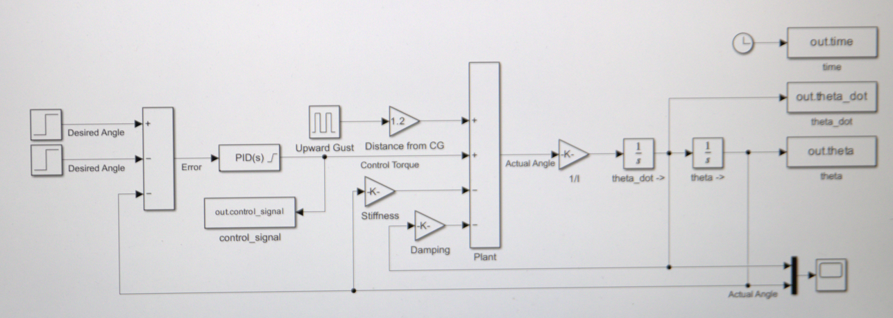
Simulink Model of PID Pitch Stabilization — **Figure 2:** Simulink model of PID-controlled pitch response under control and disturbance inputs.

The system’s main signal flow can be summarized as follows:

Step Input Block
- Step time: 1 second
- Initial value: 0°
- Final value: 10° (or 0.1745 radians used in the step block)
PID Controller Block
- Proportional gain (P): varies by test case
- Integral gain (I): varies by test case
- Derivative gain (D): varies by test case
- Filter coefficient: Tuned for smoothing if needed
Gain Block (1/I)
- Calculated moment of inertia: I = 12,182 kg·m²
- Gain value: 1 / 12,182 ≈ 8.21 × 10⁻⁵ (1 / N·m·s²)
Damping Gain Block (D)
- Gain: 510,507 N·m·s/rad
Stiffness Gain Block (K)
- Gain: 729,296 N·m/rad
Integrator Blocks (2 total)
- Initial condition: 0 (for both angular velocity and angular displacement)
To Workspace Blocks
- Save format: Array
- Variable names: e.g., theta, theta_dot, control_signal
- Limit data points: Unchecked (records entire sim duration)
Disturbance Torque (Pulse Generator and Gain)
- Amplitude: 560.2 N·m
- Period: 30 seconds
- Pulse width: 16.6% (5 seconds)
- Phase delay: 1 second

These parameter values represent estimated physical properties and control assumptions based on AH-1 Cobra dynamics and control theory.

With all variables and parameters defined, simulation can begin.

Work in Progress Below

Roadmap to Conclusion

Section	Purpose
Flight-Test Strategy	Outline test objectives, manoeuvre sequence, and safety limits that will validate the simulation results on the aircraft.
Instrumentation & Data Capture	Describe the sensors, data-rates, and logging hardware required to measure pitch response in flight.
Model Validation & System ID	Compare flight-test data with simulated response and refine model parameters using system-identification techniques.
Results Analysis	Interpret time-domain and frequency-domain metrics, highlight discrepancies, and discuss control-margin implications.
Conclusions & Recommendations	Summarise findings, state limitations, and recommend next steps for full-envelope testing or design updates.
Final Publication	Package the report, web page, and presentation materials for external review and professional outreach.